Agricultural planning doesn’t have to be complicated. Linear production models are the workhorses of farm management—straightforward, practical, and surprisingly effective. These models assume a direct, proportional relationship between inputs and outputs.

Picture this: for every pound of fertilizer you add, you get an additional 8 pounds of corn. Simple, right? That’s linear thinking in action.

The beauty lies in the simplicity:

Y = a + bX

Where Y is your yield, X is your input (like fertilizer, labor hours, or water), a is your baseline yield, and b is the constant rate of return.

Farmers love these models because they:

• Make budget planning straightforward

• Allow quick calculations in the field

• Help with resource allocation decisions

• Provide clear breakeven points

Most useful when you’re dealing with limited resource ranges or when you need a quick estimate. They won’t capture all the complexities, but they’ll get you 80% of the way there with 20% of the effort.

When and why to use quadratic production functions

Linear models are nice, but let’s get real—agriculture rarely follows a straight line. That’s where quadratic models step in, capturing what happens when more isn’t always better.

The quadratic function looks like this:

Y = a + bX + cX²

That little X² makes all the difference. It’s how we mathematically express what every farmer knows instinctively—returns eventually diminish.

Use quadratic models when:

• You need to find the optimal input level (not just “more is better”)

• Your crops or livestock show diminishing returns

• You’re planning investments over a wider input range

• Environmental factors create output ceilings

Example: A farmer might find that wheat yield increases with nitrogen fertilizer up to a point, then plateaus or even decreases with excessive application. Only a quadratic model captures this relationship accurately.

Visualizing diminishing returns in crop and livestock production

Diminishing returns aren’t just theoretical—they’re the daily reality of farming. Let’s see how this plays out.

In crop production, the classic example is fertilizer response. The first 50 pounds per acre might boost corn yield by 40 bushels. The next 50 pounds? Maybe only 25 more bushels. And the next 50? Perhaps just 10 bushels more.

For livestock, feed conversion follows the same pattern. Young animals convert feed to weight gain efficiently, but as they mature, each additional pound of feed produces less additional weight.

This visualization makes it clear:

Input Level	Linear Model Prediction	Quadratic Model Prediction	Actual Farm Results
Low	50 units	48 units	49 units
Medium	100 units	85 units	82 units
High	150 units	110 units	105 units
Very High	200 units	120 units	115 units

The gap between the linear prediction and reality widens as input increases—that’s diminishing returns in action.

Comparing model accuracy in different agricultural contexts

Not all farming operations behave the same way. The model that works for Iowa corn might fail for California almonds.

Annual crops often show more pronounced diminishing returns than perennial crops. Livestock production systems vary based on animal age, breed, and management intensity.

Here’s how different models perform across agricultural contexts:

Production System	Best-Fit Model	Why It Works
Field crops (grain)	Quadratic	Clear diminishing returns with fertilizer
Vegetable production	Linear/Quad hybrid	Linear in some ranges, quadratic in others
Dairy production	Quadratic	Feed conversion efficiency decreases
Poultry (meat)	Linear	More consistent returns within typical ranges
Orchard crops	Complex nonlinear	Age-dependent yield responses

The model choice matters most when you’re near the inflection point—where returns start diminishing significantly. Get it wrong, and you could waste thousands on inputs that won’t pay back.

Smart farmers don’t just pick a model and stick with it blindly. They test, adjust, and refine based on their specific conditions. And sometimes, the simplest model that captures the essential relationship is still the best choice.

How increasing inputs eventually leads to smaller output gains

Farmers have known this truth forever, but economists gave it a fancy name: the law of diminishing returns. It’s pretty simple really.

At first, adding more fertilizer to your corn field will dramatically increase your yield. Your crops were hungry! But keep pouring on that fertilizer and eventually each additional bag gives you fewer extra bushels than the last.

Think about it like this: If your soil has zero nitrogen, adding some will cause plants to explode with growth. But once your soil has adequate nitrogen, adding more won’t help much – and might even hurt yields.

This applies to every farm input:

• Water: Perfect amount makes crops thrive; too much drowns them

• Labor: One worker per acre? Great! Ten workers per acre? They’re just standing around

• Machinery: Right-sized equipment boosts efficiency; oversized equipment wastes money

• Seeds: Optimal plant density maximizes yield; overcrowding creates competition

The math behind this is straightforward. Your production function might look like:
Yield = 10X – 0.5X², where X is fertilizer amount

Using calculus, we can find that maximum yield occurs at X = 10. Any more fertilizer actually reduces output!

Identifying the optimal level of fertilizer, water, and labor inputs

Finding the sweet spot for each input isn’t guesswork anymore. Smart farmers use data to pinpoint exactly when adding more stops making economic sense.

For fertilizer, soil tests tell you what’s already there, and crop removal rates show what you’ll need to replace. The optimal level is where the value of yield increase equals the cost of additional fertilizer – not a pound more.

Let’s break down a real example:

Nitrogen (lbs/acre)	Corn Yield (bu/acre)	Marginal Yield Increase	Value of Increase ($)	Cost of N ($)	Net Return ($)
0	125	–	–	0	–
50	155	30	150	35	115
100	175	20	100	35	65
150	185	10	50	35	15
200	188	3	15	35	-20

See that? At 200 pounds of nitrogen, the farmer actually loses money!

Water optimization works similarly but requires monitoring soil moisture and plant stress. Technologies like soil moisture sensors and evapotranspiration models help determine precise irrigation timing and amounts.

Labor optimization gets trickier with seasonal demands. During critical periods like planting and harvest, the value of additional workers stays high longer. During maintenance periods, the optimal labor level drops significantly.

Real farm case studies demonstrating diminishing returns

A potato farm in Idaho documented their experience with irrigation precision perfectly. When they moved from traditional flood irrigation to center pivot systems, their yields jumped 22%. Adding soil moisture sensors boosted yields another 8%. But when they invested in variable rate irrigation technology, yields only improved by 3% – not enough to justify the expense.

The Wright family dairy in Wisconsin tracked labor efficiency meticulously. Their first three employees each managed 40 cows. The next three managed 35 cows each. By the time they hired their tenth employee, that person could only handle 20 cows efficiently. The operation hit classic diminishing returns.

Diminishing returns show up clearly in fertilizer trials too. A Kansas wheat farmer’s field trials revealed:

• First 30 lbs of phosphorus: 12 bushel increase

• Second 30 lbs of phosphorus: 5 bushel increase

• Third 30 lbs of phosphorus: 1 bushel increase

Modern precision ag companies have mountains of this data. One major study across 5,000 corn fields showed that nitrogen application follows a clear diminishing returns curve, with optimal rates varying by soil type, previous crop, and weather conditions.

Strategies to postpone the point of diminishing returns

Smart farmers don’t just accept diminishing returns – they fight them. The goal is pushing that inflection point further out so you can keep growing efficiently.

Precision agriculture is the biggest weapon in this battle. By applying inputs exactly where and when needed, you avoid wasting resources on areas that won’t respond. Variable rate technology means your sprayer applies more fertilizer on poor soil areas and less on naturally rich spots.

Crop rotation brilliantly resets diminishing returns cycles. Corn depletes certain nutrients while fixing others. Follow with soybeans, and you’ve essentially “refilled the tank” for specific resources.

Genetic improvements constantly push the curve outward. Modern corn hybrids respond to higher plant populations without the yield penalties older varieties would show.

Cover crops work wonders too. They capture nutrients that would otherwise leach away and make them available to the next cash crop, effectively increasing the efficiency of your previous fertilizer application.

Conservation tillage preserves soil structure and organic matter, improving water infiltration and retention. This extends the productive response curve for both water and nutrients.

The most progressive farmers now use biological amendments and soil health approaches to fundamentally change their soil’s ability to utilize inputs. Building soil biology creates new pathways for nutrient cycling that weren’t previously available.

The simple truth? You can’t escape diminishing returns entirely, but with the right strategies, you can stay in the “sweet spot” of your production function much longer.

FAQs

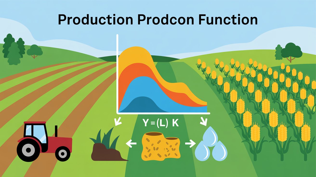
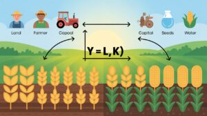
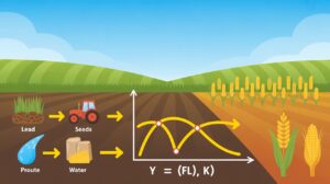
Q1: What is an agricultural production function?

A: An agricultural production function shows the relationship between inputs (like land, labor, and capital) and the resulting agrarian output.

Q2: Why is the production function important in agriculture?

A: It helps farmers and economists understand how to use resources efficiently to maximize crop yields and reduce costs.

Q3: What are the main inputs in an agricultural production function?

A: Common inputs include land, labor, capital (like tractors), seeds, water, and fertilizers.

Q4: What is the basic form of the production function?

A: A simple form is Y = f(L, K), where Y is output, L is labor, and K is capital. It can also include land and other inputs.

Q5: Can production functions be used to predict yields?

A: Yes, they help predict how changes in input levels affect output, which supports better decision-making in farm management.

Q6: Are there different types of production functions in agriculture?

A: Yes, common types include linear, Cobb-Douglas, and quadratic production functions, each with different mathematical properties.

---

Q5: Can production functions be used to predict yields?
A: Yes, they help predict how changes in input levels affect output, which supports better decision-making in farm management.

---

Q6: Are there different types of production functions in agriculture?
A: Yes, common types include linear, Cobb-Douglas, and quadratic production functions, each with different mathematical properties.

For more information